Annotab Studio 2.0.0 is now live
Lost in mAP: A Journey through Mean Average Precision in Object Detection
Lost in mAP: A Journey through Mean Average Precision in Object Detection
Lost in mAP: A Journey through Mean Average Precision in Object Detection
Lost in mAP: A Journey through Mean Average Precision in Object Detection
Published by

Dao Pham
on
Oct 3, 2023
under
Computer Vision
Published by
Dao Pham
on
Oct 3, 2023
under
Computer Vision
Published by
Dao Pham
on
Oct 3, 2023
under
Computer Vision
Published by
Dao Pham
on
Oct 3, 2023
under
Computer Vision
ON THIS PAGE
Tl;dr
A step-by-step introduction to mean average precision and how it works.
Tl;dr
A step-by-step introduction to mean average precision and how it works.
Tl;dr
A step-by-step introduction to mean average precision and how it works.
Tl;dr
A step-by-step introduction to mean average precision and how it works.

Introduction
As a newbie to the field of deep learning, you embark on your initial step in object detection. Learning the ropes of building an object detection model can be a challenging endeavor. After investing significant effort in understanding the techniques involved, you eventually manage to successfully implement them. The sense of accomplishment fills you with joy, but there's still an essential aspect you cannot overlook: Evaluating the model's performance! The widely recognized metric for this purpose is mean Average Precision (mAP). This metric plays an essential role in assessing the effectiveness of object detection models.
You tried to read many documents about mAP, but... you felt concerned about something not being clear and perhaps got lost in it. Although it is difficult, you haven't given up and want to continue. Don't worry! You're not flying solo! This article aims to help you understand this topic from scratch: from what mean average precision is to how it works. Let’s get started!
What is object detection?
Now, let’s take an overview of object detection and its applications. Object detection is a computer vision technique that combines two tasks: Localizing and identifying objects of interest in images or video frames.
Localizing is the process of determining the location or coordinate of objects. In other words, it answers the question: "Where is the object in the image?".
Identifying is the task of recognizing or classifying the object once it has been localized. It addresses the inquiry: "What is the object? What category or class does it belong to?"
Object detection is a fundamental component of the visual problem in AI and this technology has a wide range of applications:
Self-driving: This is an object detection-based method. Information is gathered from the surrounding environment by various sensors such as cameras, LiDAR, radar, GPS, temperature, and weather sensors,… These sensors provide crucial inputs: other vehicles, pedestrians, traffic signs, and obstacles,… Object detection allows autonomous vehicles to perceive, and decision-making systems are built upon this perception, enabling them to interact with the environment effectively.
Security: Object detection plays a crucial role in this application. Firstly, it is used for access control through face recognition. In detail, it identifies criminals, unauthorized accesses, or suspicious activities through CCTV cameras. Furthermore, it is useful for the early detection of fire and smoke, along with the analysis of crowd behavior in public spaces. In summary, object detection strengthens security systems to identify and respond to potential threats swiftly and effectively.
Retail: Object detection enhances the management process, with one popular application being cashier-less systems. This function allows customers to self-checkout, where products are automatically identified and the bill is also calculated. Another benefit is checking the effective placement of products, including identifying products that are out of stock or incorrectly positioned.
Healthcare: The well-known usage is face mask recognition during the COVID-19 pandemic. Additionally, object detection is not only used for detecting harmful areas such as tumors or disease regions but is also valuable for tracking the movement of objects of interest. This technology aids radiologists and clinicians in faster and more accurate disease detection and diagnosis. Moreover, object detection can monitor patients and provide early fall detection.

Figure 1: Example of applications of object detection in self-driving, healthcare and retail
Before we dive deep into mAP, let's thoroughly explore some related definitions: confusion matrix and Intersection over Union (IoU).
What is object detection?
Now, let’s take an overview of object detection and its applications. Object detection is a computer vision technique that combines two tasks: Localizing and identifying objects of interest in images or video frames.
Localizing is the process of determining the location or coordinate of objects. In other words, it answers the question: "Where is the object in the image?".
Identifying is the task of recognizing or classifying the object once it has been localized. It addresses the inquiry: "What is the object? What category or class does it belong to?"
Object detection is a fundamental component of the visual problem in AI and this technology has a wide range of applications:
Self-driving: This is an object detection-based method. Information is gathered from the surrounding environment by various sensors such as cameras, LiDAR, radar, GPS, temperature, and weather sensors,… These sensors provide crucial inputs: other vehicles, pedestrians, traffic signs, and obstacles,… Object detection allows autonomous vehicles to perceive, and decision-making systems are built upon this perception, enabling them to interact with the environment effectively.
Security: Object detection plays a crucial role in this application. Firstly, it is used for access control through face recognition. In detail, it identifies criminals, unauthorized accesses, or suspicious activities through CCTV cameras. Furthermore, it is useful for the early detection of fire and smoke, along with the analysis of crowd behavior in public spaces. In summary, object detection strengthens security systems to identify and respond to potential threats swiftly and effectively.
Retail: Object detection enhances the management process, with one popular application being cashier-less systems. This function allows customers to self-checkout, where products are automatically identified and the bill is also calculated. Another benefit is checking the effective placement of products, including identifying products that are out of stock or incorrectly positioned.
Healthcare: The well-known usage is face mask recognition during the COVID-19 pandemic. Additionally, object detection is not only used for detecting harmful areas such as tumors or disease regions but is also valuable for tracking the movement of objects of interest. This technology aids radiologists and clinicians in faster and more accurate disease detection and diagnosis. Moreover, object detection can monitor patients and provide early fall detection.
Figure 1: Example of applications of object detection in self-driving, healthcare and retail
Before we dive deep into mAP, let's thoroughly explore some related definitions: confusion matrix and Intersection over Union (IoU).
Clarification of the confusion in confusion matrix
Ground truths and predictions
In most cases, you need a labeled dataset to build an object detection model. Labeling involves annotating each image in the dataset to specify the location and category (a class) of interested objects you want the model to detect. This information is crucial for training the model because it allows the model to learn patterns and features associated with different objects‘s categories and their positions. Bounding box is one of the types of annotations commonly used in object detection. This is a rectangular area of an image containing the object of the class to be detected. It is called a ‘ground truth bounding box’ or ‘actual bounding box’, simply are ‘ground truth box’ or ‘actual box’.
The output of detection model consists of a bounding box, a class, and a confidence value. The predicted bounding box made by model is simply named ‘predicted box’.
In Figure 3, these green boxes are actual boxes and pink boxes are predicted boxes made by the model.
Precision and Recall
First of all, let’s talk about “positive” and “negative” in the context of object detection.
“Positive” typically represents to object of interest – it means a class we want to detect. When we have multiple classes, each class is considered “positive” sequentially, and the rest are considered “negative”.
“Negative" refers to a bounding box or region that does not contain the target class. It can be other classes or regions that do not cover the target class. Simply, negatives are the rest of the image except for the positives.
Following these definitions, "positive" and "negative" help clarify the difference between detecting the object of interest and what is not the object in object detection scenarios.
True positive: The detection is identified as positive and it is truly positive.
False positive: The detection is identified as positive but it's actually a negative.
True negative: The detection is identified as negative and it is truly negative.
False negative: The detection is identified as negative but it's actually a positive.
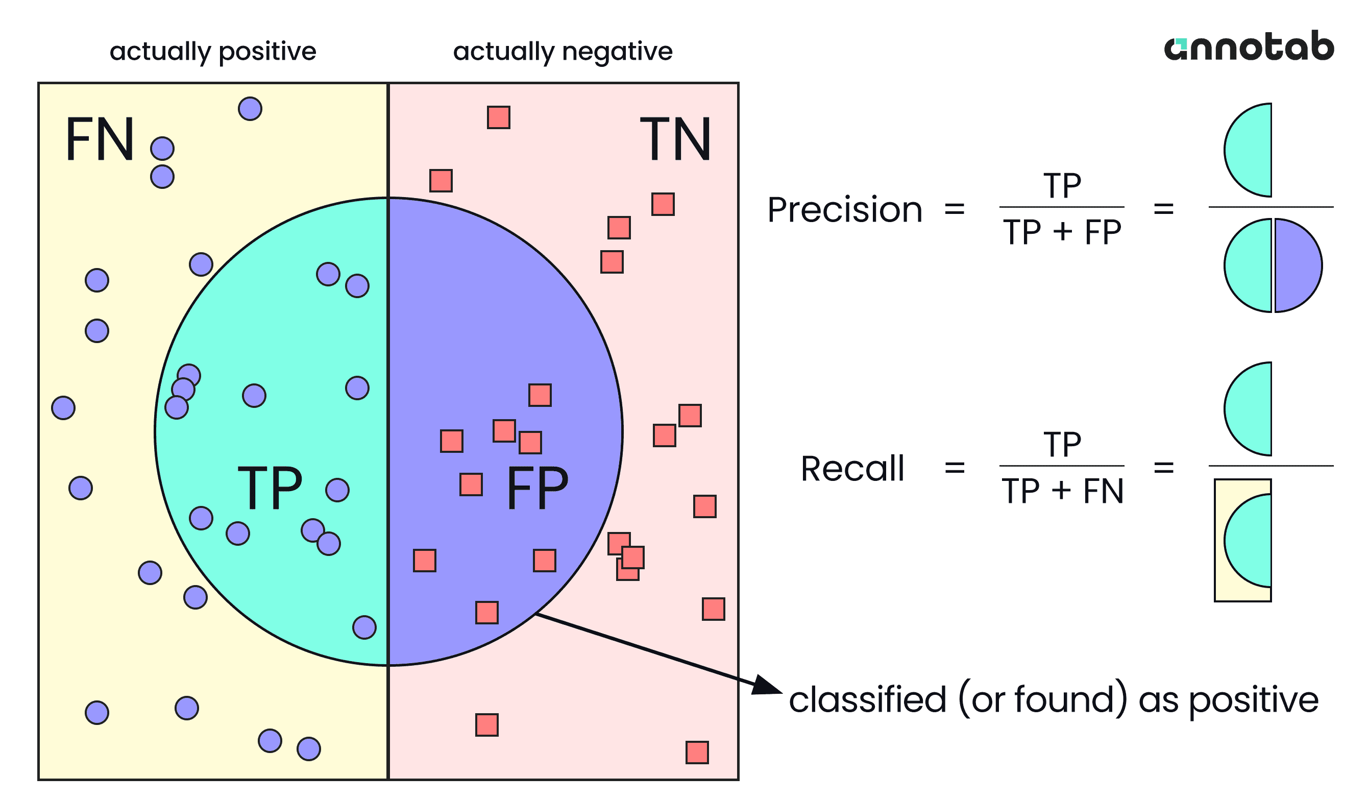
Figure 2: Visualization of True positive, False positive, True negative, False negative
Precision and recall are typically calculated for each class separately. This allows you to evaluate the model's performance for each individual class in terms of its ability to correctly detect and classify objects of that class.
Precision is the ratio of true positive detections (TP) to the total number of positive detections the model made (TP+FP). It measures how accurate detection is. i.e. the percentage of detections that are correct.
Recall is the ratio of true positive detections (TP) to the total number of all actual positives (all actual positives = total number of ground truth = TP + FN). On the other hand, Recall measures how well the model finds all the positives.
Ok, let’s take a basic example. Assume we have a dog detection model, and we evaluate it on this image:

Figure 3: Predicted boxes and ground truth boxes by dog detection model
+ Number of true positives = 4
+ Number of false positives = 1
+ Number of false negative = 0
As you can see, while the Recall is 1, the Precision is 0.8. It means the model succeeds in detecting all the dogs, but it is also incorrect in detecting some cases.
Intersection over Union (IoU)
The IoU measures the overlap between the predicted bounding box (the region the model believes contains the object) and the ground truth bounding box (the actual region where the object is located).
It is calculated as the ratio of the area of intersection (the overlapping region) to the area of the union of the predicted and ground truth bounding boxes.

Figure 4: Intersection over Union
The value of IoU ranges from 0 to 1, where:
+ IoU = 0: No overlapping between the predicted and ground truth bounding box.
+ IoU ≈ 1: Perfect matching between the predicted and ground truth bounding boxes, meaning they nearly completely overlap.
In section 2, we discuss precision and recall without the context of IoU. However, object detection requires to use the IoU value as a measurement when identifying true positives and false positives. In general, the common value used for IoU is 0.5, 0.75 or 0.9,… depending on individual purposes.
For example, when you choose an IoU value of 0.5, it means that only the predicted bounding boxes whose IoU with their respective ground truth bounding boxes is equal to or greater than 0.5 are considered true positives. If the IoU is smaller than 0.5, they are considered as false positives.

Figure 5: Example of determining true positives based on IoU
Look at the Husky’s image, assume the IoU of the predicted box and ground truth box is 0.72.
If the IoU threshold is 0.7, this predicted box is considered true positive. But if we choose the IoU threshold as 0.75, it becomes a false positive.
So, based on the definition of object detection, when a predicted bounding box is ‘false positive’, it can be:
+ Correctly predict the category or class it belongs to, but have an IoU with its ground truth box smaller than the IoU threshold (localization issue)
+ Have an IoU with its ground truth box greater than the IoU threshold but incorrectly predict its category or class (identification issue).
Clarification of the confusion in confusion matrix
Ground truths and predictions
In most cases, you need a labeled dataset to build an object detection model. Labeling involves annotating each image in the dataset to specify the location and category (a class) of interested objects you want the model to detect. This information is crucial for training the model because it allows the model to learn patterns and features associated with different objects‘s categories and their positions. Bounding box is one of the types of annotations commonly used in object detection. This is a rectangular area of an image containing the object of the class to be detected. It is called a ‘ground truth bounding box’ or ‘actual bounding box’, simply are ‘ground truth box’ or ‘actual box’.
The output of detection model consists of a bounding box, a class, and a confidence value. The predicted bounding box made by model is simply named ‘predicted box’.
In Figure 3, these green boxes are actual boxes and pink boxes are predicted boxes made by the model.
Precision and Recall
First of all, let’s talk about “positive” and “negative” in the context of object detection.
“Positive” typically represents to object of interest – it means a class we want to detect. When we have multiple classes, each class is considered “positive” sequentially, and the rest are considered “negative”.
“Negative" refers to a bounding box or region that does not contain the target class. It can be other classes or regions that do not cover the target class. Simply, negatives are the rest of the image except for the positives.
Following these definitions, "positive" and "negative" help clarify the difference between detecting the object of interest and what is not the object in object detection scenarios.
True positive: The detection is identified as positive and it is truly positive.
False positive: The detection is identified as positive but it's actually a negative.
True negative: The detection is identified as negative and it is truly negative.
False negative: The detection is identified as negative but it's actually a positive.
Figure 2: Visualization of True positive, False positive, True negative, False negative
Precision and recall are typically calculated for each class separately. This allows you to evaluate the model's performance for each individual class in terms of its ability to correctly detect and classify objects of that class.
Precision is the ratio of true positive detections (TP) to the total number of positive detections the model made (TP+FP). It measures how accurate detection is. i.e. the percentage of detections that are correct.
Recall is the ratio of true positive detections (TP) to the total number of all actual positives (all actual positives = total number of ground truth = TP + FN). On the other hand, Recall measures how well the model finds all the positives.
Ok, let’s take a basic example. Assume we have a dog detection model, and we evaluate it on this image:
Figure 3: Predicted boxes and ground truth boxes by dog detection model
+ Number of true positives = 4
+ Number of false positives = 1
+ Number of false negative = 0
As you can see, while the Recall is 1, the Precision is 0.8. It means the model succeeds in detecting all the dogs, but it is also incorrect in detecting some cases.
Intersection over Union (IoU)
The IoU measures the overlap between the predicted bounding box (the region the model believes contains the object) and the ground truth bounding box (the actual region where the object is located).
It is calculated as the ratio of the area of intersection (the overlapping region) to the area of the union of the predicted and ground truth bounding boxes.
Figure 4: Intersection over Union
The value of IoU ranges from 0 to 1, where:
+ IoU = 0: No overlapping between the predicted and ground truth bounding box.
+ IoU ≈ 1: Perfect matching between the predicted and ground truth bounding boxes, meaning they nearly completely overlap.
In section 2, we discuss precision and recall without the context of IoU. However, object detection requires to use the IoU value as a measurement when identifying true positives and false positives. In general, the common value used for IoU is 0.5, 0.75 or 0.9,… depending on individual purposes.
For example, when you choose an IoU value of 0.5, it means that only the predicted bounding boxes whose IoU with their respective ground truth bounding boxes is equal to or greater than 0.5 are considered true positives. If the IoU is smaller than 0.5, they are considered as false positives.
Figure 5: Example of determining true positives based on IoU
Look at the Husky’s image, assume the IoU of the predicted box and ground truth box is 0.72.
If the IoU threshold is 0.7, this predicted box is considered true positive. But if we choose the IoU threshold as 0.75, it becomes a false positive.
So, based on the definition of object detection, when a predicted bounding box is ‘false positive’, it can be:
+ Correctly predict the category or class it belongs to, but have an IoU with its ground truth box smaller than the IoU threshold (localization issue)
+ Have an IoU with its ground truth box greater than the IoU threshold but incorrectly predict its category or class (identification issue).
Mean Average Precision (mAP)
Now, let's discuss our main character in this article: mAP. Noting again, we work with each class in a multi-class object detection sequentially.
Precision-Recall curve (PR curve)
First, we will explore the concept of the PR curve.
As I mentioned above, the output of the object detection model are: predicted bounding box, a class, and a confidence value. A confidence value tells us how the model is confident with its detection. Detection whose confidence value is greater than a threshold is considered as positive (It can be true or false positive).
The Precision-Recall (PR) curve in object detection is typically created by many pairs of precision-recall at various confidence thresholds. Each precision-recall pair is computed for a given confidence threshold. When the confidence threshold decreases, the number of detections increases. It means we have more true and false positives. The more true positive, the higher Recall. Let’s take a mathematical explanation.
The equation of Recall:
The denominator is fixed because the number of ground truths doesn’t change. Since we have more true positives, the Recall increases.
So, how about the Precision? Both the numerator and denominator of the precision equation are increased. Since, the Precision can be increased, decreased or unchanged. Therefore, the PR curve is a zig-zag function.
In general, the trend of Precision can be a negative slope. The reason is that when the confidence threshold decreases, the model has less confidence about the detections it makes, causing more false positives to occur at low confidence. Therefore, the possibility of those detections being false positives is high, and the possibility of them being true positives is low. So, in this case, Precision can decrease. (1)

However, there is no guarantee of that, as there is also a situation where some detections have low confidence but are actually true positives. When confidence drops, Precision will increase. (2).

In summary, precision can either decrease, increase, or stay unchanged when confidence decreases. However, in most cases, situation (1) occurs more frequently than (2), so the trend of precision seems to be a decreasing behavior.

Figure 6: Precision-Recall trade-off
Average Precision (AP) and mean Average Precision (mAP)
An ideal object detector should not miss any ground-truth objects (FN = 0) and detect only relevant objects (FP = 0). In general, an object detector can be considered good if when the confidence threshold decreases, its precision stays high while its recall increases (the number of true positives grows, the number of false positives unchanged or increase by a very small amount), which means the precision and recall still be high at varying confidence threshold. As a result, the area under the curve (AUC) is large when both precision and recall are high.
A poor object detector can be:
High Precision, Low Recall: In the scenario, where an object detector finds only one or a few true positives with high confidence, it results in high Precision because the number of false positives is either zero or very small. However, this also means that the Recall is very low because the model is missing many true positive objects. This situation is common when the model is very conservative and only makes predictions when it is highly confident, often resulting in missed detections.
High Recall, Low Precision: Conversely, when a model predicts many detections, it means including a lot of false positives. Leading to high recall because it captures most of the true positive objects. However, the Precision in this case is low because there are many false positives among the detections. This situation occurs when the model is less conservative and makes more detections, but it also makes more mistakes in the form of false positives.
In object detection, the average precision (AP) is the area under the PR curve. One class has its own average precision. The mAP is the average of the AP calculated for all the classes. Assume we have C class, the formula of mAP:
Mean average precision (mAP) is one of the metrics used for evaluating the performance of object detection model by providing an overview of the sensitivity of the model. mAP@0.5 means that is a mAP calculated at IoU threshold 0.5. mAP@[.5:.05:.95] is computed at the 10 IoU threshold from 0.5 to 0.95 with step = 0.05, and then get the average of all results.
A good mAP indicates a model that's stable and consistent across different confidence thresholds. So, to compute mAP, we first find the AP value for each class by calculating the AUC of its PR curve. In general, the PR curve does not exhibit a monotonic behavior; it is zig-zag instead. Therefore, before computing AP, precision-recall pairs have to be interpolated. The interpolated Precision at a Recall R ∈[0,1] is determined by this equation:
An interpolated precision at a given recall R is the maximum precision obtained from the remaining precisions, where their corresponding recall is equal to or greater than R.
After the interpolation process, we have a new set of interpolated precision. The AP is the area under the new PR curve and is calculated by using the Riemann sum approximation.
Assume:
We have K confidence thresholds
The confidence threshold at k+1 > confidence threshold at k
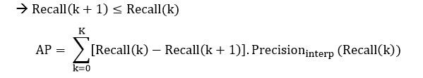
There are two approaches to compute this Riemann integral: The N-point interpolation and the all-point interpolation.
N-point interpolation:
Now, let’s analyze a numerical example.Popular applications of this interpolation method use N = 11 or N = 101
All-point interpolation:
The set values of Recall(n), Recall(n+1)… Recall(n) used to compute the AP corresponds exactly to the set of original Recall values.
Now, let’s analyze a numerical example.
We've got a model for dog detection, and it's telling us it found 15 dogs (The number of ground truth dogs is 17). Those predicted dogs are in pink boxes, and each box has a letter from 'A' to 'O' on it. In each box, there is a number that shows us how confident the model is about finding the dog. As we can see, the model either successfully detects some dogs, misses some of them, or is also incorrect in detecting them.
First, we sort those detections by their confidence levels in descending. After that, we determine whether they are true or false positives and calculate the precision and recall.
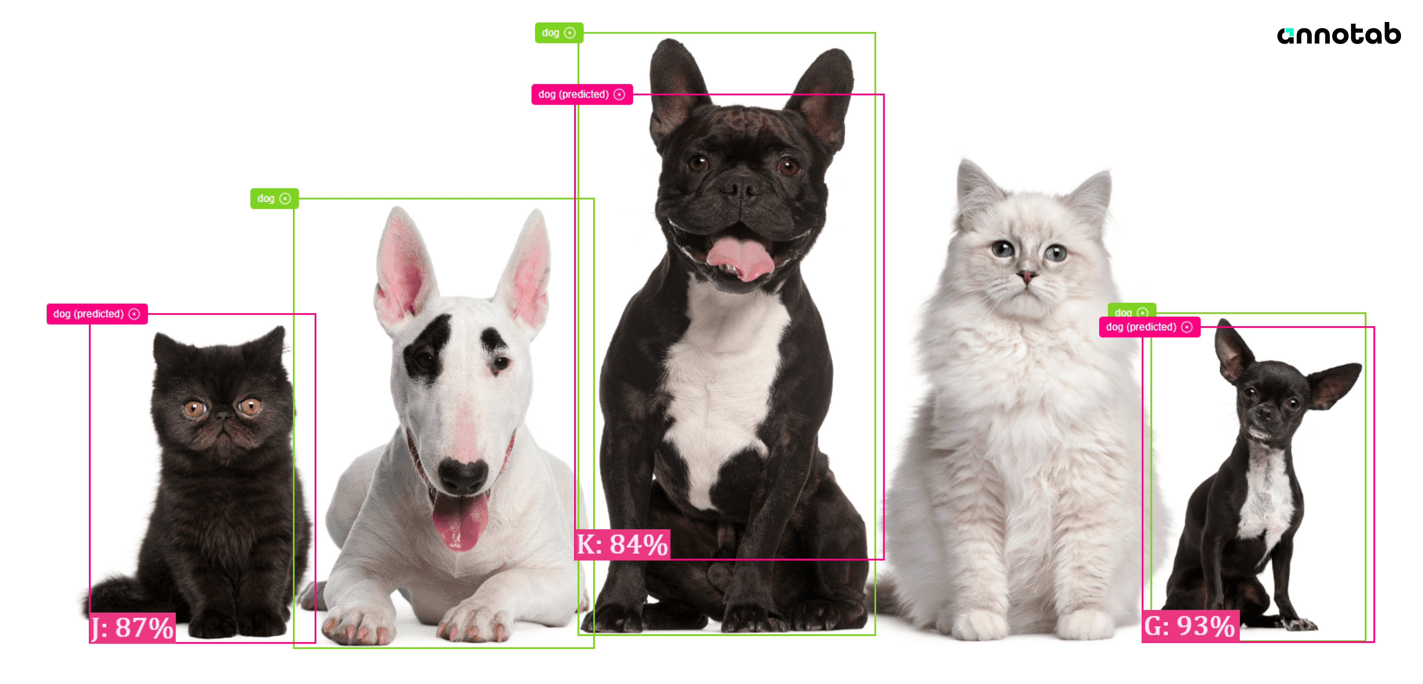


We choose IoU threshold = 0.5 in this example.
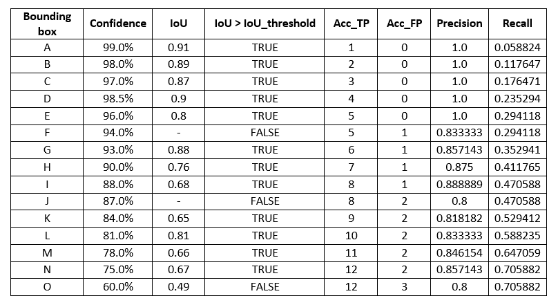
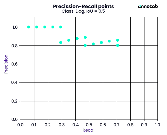
Figure 7: Precision-Recall points in class ‘Dog’ with IoU threshold = 0.5
Let’s calculate the average precision (AP)!
11-point interpolation:
Recall = [0.0, 0.1, 0.2, 0.3, 0.4, 0.5, 0.6, 0.7, 0.8, 0.9, 1.0]Recall = 0.0, original Recalls that equal to greater than it: [0. 058824, 0.117647, …, 0.705882] ≥ 0.0; their correspond Precisions = [1.0, 1.0, …, 0.8]; max of those Precisions = 1.0. We have the first pair precision-recall = (1.0, 0.1)
Recall = 0.1, original Recalls that equal to greater than it: [0.117647, 0.176471 …, 0.705882] ≥ 0.1; their corresponding Precisions = [1.0, 1.0, …, 0.8]; max of those Precisions = 1.0. We have the second pair precision-recall = (1.0, 0.1)
Recall = 0.2, original Recalls that equal to greater than it: [0.235294, 0.294118…, 0.705882] ≥ 0.2; their correspond Precisions = [1.0, 1.0, …, 0.8]; max of those Precisions = 1.0. We have the third pair precision-recall = (1.0, 0.2)
Recall = 0.3, original Recalls that equal to greater than it: [0.352941, 0.411765…, 0.705882] ≥ 0.3; their corresponding Precisions = [0.857143, 0.875, …, 0.8]; max of those Precisions = 0.888889. We have the fourth pair precision-recall = (0.888889, 0.3)
…
Recall = 0.8, original Recalls that equal to greater than it: {∅}; their corresponding Precisions = {∅}; max of those Precisions = 0. Precision-recall = (0.0, 0.0)
…
Recall = 1.0, original Recalls that equal to greater than it: {∅}; their corresponding Precisions = {∅}; max of those Precisions = 0. Precision-recall = (0.0, 0.0)
All-point interpolation:
It is a homework for you. (hint: AP≈0.6527)
Mean Average Precision (mAP)
Now, let's discuss our main character in this article: mAP. Noting again, we work with each class in a multi-class object detection sequentially.
Precision-Recall curve (PR curve)
First, we will explore the concept of the PR curve.
As I mentioned above, the output of the object detection model are: predicted bounding box, a class, and a confidence value. A confidence value tells us how the model is confident with its detection. Detection whose confidence value is greater than a threshold is considered as positive (It can be true or false positive).
The Precision-Recall (PR) curve in object detection is typically created by many pairs of precision-recall at various confidence thresholds. Each precision-recall pair is computed for a given confidence threshold. When the confidence threshold decreases, the number of detections increases. It means we have more true and false positives. The more true positive, the higher Recall. Let’s take a mathematical explanation.
The equation of Recall:
The denominator is fixed because the number of ground truths doesn’t change. Since we have more true positives, the Recall increases.
So, how about the Precision? Both the numerator and denominator of the precision equation are increased. Since, the Precision can be increased, decreased or unchanged. Therefore, the PR curve is a zig-zag function.
In general, the trend of Precision can be a negative slope. The reason is that when the confidence threshold decreases, the model has less confidence about the detections it makes, causing more false positives to occur at low confidence. Therefore, the possibility of those detections being false positives is high, and the possibility of them being true positives is low. So, in this case, Precision can decrease. (1)
However, there is no guarantee of that, as there is also a situation where some detections have low confidence but are actually true positives. When confidence drops, Precision will increase. (2).
In summary, precision can either decrease, increase, or stay unchanged when confidence decreases. However, in most cases, situation (1) occurs more frequently than (2), so the trend of precision seems to be a decreasing behavior.
Figure 6: Precision-Recall trade-off
Average Precision (AP) and mean Average Precision (mAP)
An ideal object detector should not miss any ground-truth objects (FN = 0) and detect only relevant objects (FP = 0). In general, an object detector can be considered good if when the confidence threshold decreases, its precision stays high while its recall increases (the number of true positives grows, the number of false positives unchanged or increase by a very small amount), which means the precision and recall still be high at varying confidence threshold. As a result, the area under the curve (AUC) is large when both precision and recall are high.
A poor object detector can be:
High Precision, Low Recall: In the scenario, where an object detector finds only one or a few true positives with high confidence, it results in high Precision because the number of false positives is either zero or very small. However, this also means that the Recall is very low because the model is missing many true positive objects. This situation is common when the model is very conservative and only makes predictions when it is highly confident, often resulting in missed detections.
High Recall, Low Precision: Conversely, when a model predicts many detections, it means including a lot of false positives. Leading to high recall because it captures most of the true positive objects. However, the Precision in this case is low because there are many false positives among the detections. This situation occurs when the model is less conservative and makes more detections, but it also makes more mistakes in the form of false positives.
In object detection, the average precision (AP) is the area under the PR curve. One class has its own average precision. The mAP is the average of the AP calculated for all the classes. Assume we have C class, the formula of mAP:
Mean average precision (mAP) is one of the metrics used for evaluating the performance of object detection model by providing an overview of the sensitivity of the model. mAP@0.5 means that is a mAP calculated at IoU threshold 0.5. mAP@[.5:.05:.95] is computed at the 10 IoU threshold from 0.5 to 0.95 with step = 0.05, and then get the average of all results.
A good mAP indicates a model that's stable and consistent across different confidence thresholds. So, to compute mAP, we first find the AP value for each class by calculating the AUC of its PR curve. In general, the PR curve does not exhibit a monotonic behavior; it is zig-zag instead. Therefore, before computing AP, precision-recall pairs have to be interpolated. The interpolated Precision at a Recall R ∈[0,1] is determined by this equation:
An interpolated precision at a given recall R is the maximum precision obtained from the remaining precisions, where their corresponding recall is equal to or greater than R.
After the interpolation process, we have a new set of interpolated precision. The AP is the area under the new PR curve and is calculated by using the Riemann sum approximation.
Assume:
We have K confidence thresholds
The confidence threshold at k+1 > confidence threshold at k
There are two approaches to compute this Riemann integral: The N-point interpolation and the all-point interpolation.
N-point interpolation:
Now, let’s analyze a numerical example.Popular applications of this interpolation method use N = 11 or N = 101
All-point interpolation:
The set values of Recall(n), Recall(n+1)… Recall(n) used to compute the AP corresponds exactly to the set of original Recall values.
Now, let’s analyze a numerical example.
We've got a model for dog detection, and it's telling us it found 15 dogs (The number of ground truth dogs is 17). Those predicted dogs are in pink boxes, and each box has a letter from 'A' to 'O' on it. In each box, there is a number that shows us how confident the model is about finding the dog. As we can see, the model either successfully detects some dogs, misses some of them, or is also incorrect in detecting them.
First, we sort those detections by their confidence levels in descending. After that, we determine whether they are true or false positives and calculate the precision and recall.
We choose IoU threshold = 0.5 in this example.
Figure 7: Precision-Recall points in class ‘Dog’ with IoU threshold = 0.5
Let’s calculate the average precision (AP)!
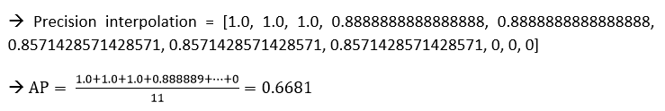
11-point interpolation:
Recall = [0.0, 0.1, 0.2, 0.3, 0.4, 0.5, 0.6, 0.7, 0.8, 0.9, 1.0]Recall = 0.0, original Recalls that equal to greater than it: [0. 058824, 0.117647, …, 0.705882] ≥ 0.0; their correspond Precisions = [1.0, 1.0, …, 0.8]; max of those Precisions = 1.0. We have the first pair precision-recall = (1.0, 0.1)
Recall = 0.1, original Recalls that equal to greater than it: [0.117647, 0.176471 …, 0.705882] ≥ 0.1; their corresponding Precisions = [1.0, 1.0, …, 0.8]; max of those Precisions = 1.0. We have the second pair precision-recall = (1.0, 0.1)
Recall = 0.2, original Recalls that equal to greater than it: [0.235294, 0.294118…, 0.705882] ≥ 0.2; their correspond Precisions = [1.0, 1.0, …, 0.8]; max of those Precisions = 1.0. We have the third pair precision-recall = (1.0, 0.2)
Recall = 0.3, original Recalls that equal to greater than it: [0.352941, 0.411765…, 0.705882] ≥ 0.3; their corresponding Precisions = [0.857143, 0.875, …, 0.8]; max of those Precisions = 0.888889. We have the fourth pair precision-recall = (0.888889, 0.3)
…
Recall = 0.8, original Recalls that equal to greater than it: {∅}; their corresponding Precisions = {∅}; max of those Precisions = 0. Precision-recall = (0.0, 0.0)
…
Recall = 1.0, original Recalls that equal to greater than it: {∅}; their corresponding Precisions = {∅}; max of those Precisions = 0. Precision-recall = (0.0, 0.0)
All-point interpolation:
It is a homework for you. (hint: AP≈0.6527)
References
Padilla, R.; Passos, W.L.; Dias, T.L.B.; Netto, S.L., da Silva, E.A.B. A Comparative Analysis of Object Detection Metrics with a Companion Open-Source Toolkit. Electronics 2021, 10, 279. https://doi.org/10.3390/electronics10030279
Read more
References
Padilla, R.; Passos, W.L.; Dias, T.L.B.; Netto, S.L., da Silva, E.A.B. A Comparative Analysis of Object Detection Metrics with a Companion Open-Source Toolkit. Electronics 2021, 10, 279. https://doi.org/10.3390/electronics10030279
Read more
References
Padilla, R.; Passos, W.L.; Dias, T.L.B.; Netto, S.L., da Silva, E.A.B. A Comparative Analysis of Object Detection Metrics with a Companion Open-Source Toolkit. Electronics 2021, 10, 279. https://doi.org/10.3390/electronics10030279
Read more
References
Padilla, R.; Passos, W.L.; Dias, T.L.B.; Netto, S.L., da Silva, E.A.B. A Comparative Analysis of Object Detection Metrics with a Companion Open-Source Toolkit. Electronics 2021, 10, 279. https://doi.org/10.3390/electronics10030279
Read more
Dao Pham
Product Developer
#TechEnthusiast #AIProductDeveloper
Dao Pham
Product Developer
#TechEnthusiast #AIProductDeveloper
Dao Pham
Product Developer
#TechEnthusiast #AIProductDeveloper
Dao Pham
Product Developer
#TechEnthusiast #AIProductDeveloper