Annotab Studio 2.0.0 is now live
From Genes to Machines: The Fascinating World of Genetic Algorithms
From Genes to Machines: The Fascinating World of Genetic Algorithms
From Genes to Machines: The Fascinating World of Genetic Algorithms
From Genes to Machines: The Fascinating World of Genetic Algorithms
Published by

Dao Pham
on
Jun 1, 2024
under
AI
Published by
Dao Pham
on
Jun 1, 2024
under
AI
Published by
Dao Pham
on
Jun 1, 2024
under
AI
Published by
Dao Pham
on
Jun 1, 2024
under
AI
ON THIS PAGE
Tl;dr
Imagine you're at the grocery store, trying to find the most efficient route to grab all your items. You want to minimize the distance you walk, but also consider grabbing some fresh produce on the way. This is a simple example of multi-objective optimization, a problem where you're looking for the best solution that considers multiple factors. Genetic algorithms (GAs) are a powerful tool inspired by biological evolution that can tackle these complex optimization challenges. In this blog, we'll delve into the fascinating world of GAs and explore how they work.

What is genetic algorithm (GA) and why do we use it?
First, let’s talk about the multi-objective optimization. Multi-objective optimization refers to finding the optimal solution involving more than one objective function that has to be optimized. For example, you open a grocery store, so what do you want? High revenue and low renting cost, low transportation cost,… Many costs (multi-objective) you need to optimize (maximize revenue, minimize renting cost and transportation costs,…)
There are some ways to solve multi-objective optimization problems using mathematical optimization methods. However, these methods can be complex and require many calculations because they find the optimal solution with many conditions. The solution space is generated by considering all cases of the first goal (for example, n1 cases), all cases of the second goal (for example, n2 cases),…, and all cases of the the last goal (for example, nm cases). We get n1. n2…nm solutions and if n,m is enough large, it causes an explosion of solution space! If we do not have enough resources and limitations in time, we cannot consider all cases. Instead, we need to find another method that can find a solution that may not be the best, but rather enough good and acceptable. A naive thought is trial and error with some solutions. So, which is the right way to do that? We cannot believe in luck and select some random solution to test... We need a smart strategy to do that. This is where the genetic algorithm comes in.
The basic principles of genetic algorithms were first published by J.H. Holland in 1962. It is a stochastic search algorithm. The main idea of this method is based on the theory of natural selection. Individuals who have good fitness are selected for reproduction. The next generation in a genetic algorithm is created through a process that mimics biological reproduction.
Encoding method
The very first step before using a GA is to determine whether your solutions can be represented as chromosomes or not. Each element in a solution is deemed as a gene in a chromosome. If the solutions can represented as chromosomes, there are some ways to encode the solution.
Binary encoding
This is the most common method. We use bits 0 and 1 to create the chromosome. Each gene in the chromosome represents particular characteristics of the solution.
For example: 110101, 010110, 001101,…
Permutation encoding (or Order encoding)
This representation is used when each element in the solution is related to another in order. The chromosome in this case is represented as a sequence of genes in a specific order. For instance, in the Travelling Salesman Problem (TSP): Given a list of cities and the distances between each pair of cities, what is the shortest possible route that visits each city exactly once and returns to the origin city? Each chromosome is a route. For example: 12345, 54321, 31254,…
Value encoding
This type of encoding is used in problems where the set of solutions is the set of values. These values are created by symbols, strings or values.

Tree encoding
Tree encoding is a powerful technique for evolving programs and other structures that can be naturally represented as tree-like hierarchies. In this approach, each chromosome within the genetic algorithm is itself a tree structure, containing elements that correspond to functions, commands, or other building blocks relevant to the problem being solved.

Example of chromosomes with tree encoding
Now, let's pay attention on the main character of this topic: The Genetic Algorithm.
Encoding method
The very first step before using a GA is to determine whether your solutions can be represented as chromosomes or not. Each element in a solution is deemed as a gene in a chromosome. If the solutions can represented as chromosomes, there are some ways to encode the solution.
Binary encoding
This is the most common method. We use bits 0 and 1 to create the chromosome. Each gene in the chromosome represents particular characteristics of the solution.
For example: 110101, 010110, 001101,…
Permutation encoding (or Order encoding)
This representation is used when each element in the solution is related to another in order. The chromosome in this case is represented as a sequence of genes in a specific order. For instance, in the Travelling Salesman Problem (TSP): Given a list of cities and the distances between each pair of cities, what is the shortest possible route that visits each city exactly once and returns to the origin city? Each chromosome is a route. For example: 12345, 54321, 31254,…
Value encoding
This type of encoding is used in problems where the set of solutions is the set of values. These values are created by symbols, strings or values.
Tree encoding
Tree encoding is a powerful technique for evolving programs and other structures that can be naturally represented as tree-like hierarchies. In this approach, each chromosome within the genetic algorithm is itself a tree structure, containing elements that correspond to functions, commands, or other building blocks relevant to the problem being solved.
Example of chromosomes with tree encoding
Now, let's pay attention on the main character of this topic: The Genetic Algorithm.
Components in Genetic Algorithm
Initial population
The population contains many chromosomes. These initial chromosomes can be:
Generated randomly in the initial step
The results of other algorithms
Obtained by experts based on some specific conditions.
The number of chromosomes in the population is based on your resources.
Fitness function
The input of this function is the chromosomes and the output is the fitness value. This value shows us how close a candidate solution is to the optimal solution of the desired problem.
The fitness value is used for:
Select individuals who are a good fit for the next generation
Check the convergence of the algorithm
Termination condition
The termination is based on one of 3 criteria:
Fitness value: Once almost all candidate solutions in the population have the same fitness value, it means the algorithm convergence to a local minimum. You can stop the process.
Running time: The GA can stop after a predefined number of iterations. This decision depends on your available resources and desired execution time.
Diversity of the population: This diversity is measured by the variance of the candidate solutions. A low variance means these candidate solutions are generally similar and clustered together (convergence to a local minimum). A high variance tells us that the solutions have higher variability, and they are generally further from the mean.
Selection
Selection mechanisms are used to select candidate solutions to crossover for the next generation based on their fitness value. In general, we select the potentially useful solutions. Individuals whose high fitness value can be chosen. But it doesn’t mean we cross-over of two chromosomes have high fitness value we can get children with a high fitness value like their parents.
There are 4 methods for selection:
Roulette wheel Selection
This is the simplest way to select some solutions. Each individual has a part in Roulette wheel. The individual’s size in Roulette wheel directs proportion with the fitness value. Every time we spin the Roulette wheel we get one individual and consider it as a selected individual for regeneration.
For example, we have 5 chromosomes with their information as the table below:
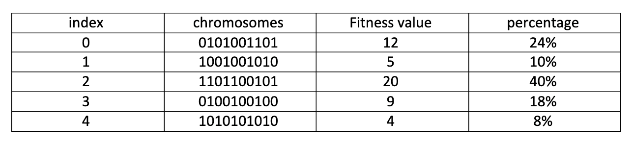
The Roulette wheel of these chromosomes is like this:

We don't need to sort the percentages because we're aiming for random selection. In this method, we spin the roulette wheel n times to select n chromosomes. The probability of selecting a chromosome is directly proportional to its fitness value. This means chromosomes with higher fitness values have a greater chance of being selected. However, this can lead to a single chromosome being selected multiple times, potentially causing premature convergence to a local minimum.
Stochastic universal sampling Selection
The idea behind this method is similar to roulette wheel selection but with an improvement. The key difference lies in using pointers. Suppose we want to select 𝑚𝑚 chromosomes from a population of 𝑛 chromosomes. The first pointer is randomly generated. Then, we select the remaining 𝑚−1 chromosomes based on the distance between pointers [Equation] on a virtual roulette wheel.
Let's take a closer look at this example:
We need to select 3 chromosomes from a population of 5 chromosomes. The distance between pointers on the virtual roulette wheel is 1313 (120 degrees). Assume the first pointer randomly lands on chromosome_3. Therefore, the remaining 2 chromosomes selected are chromosome_2 and chromosome_0.

As you can see, we randomly generate only one pointer and then can choose k individuals. This method helps reduce duplication compared to roulette wheel selection.
Linear ranking Selection
Linear ranking selection employs a sorting approach to assign fitness value ranks. Individuals within the population are first ordered based on their fitness values decreasing, with the fittest receiving rank 1, the second fittest receiving rank 2, and so on until the lowest receives rank N (population size). The second step is selection, but how do we do that?

Tournament Selection
Randomly select k individuals ( k is called the tour size) and compare their fitness. The individual with the highest or lowest fitness or any standard based on your decision is chosen in each tour. This process is repeated n times with n as the number of individuals to be selected.
Crossover
Inspired by how genes mix in nature, genetic algorithms use crossover (also known as recombination) to generate new offspring from the genetic information of parents.
Linear crossover
This method is used for chromosome representation as a binary string.
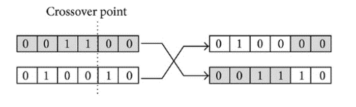
1-point crossover
A random 'crossover point' is selected on both parents' chromosomes. At this point, the bits to the right are exchanged between the two parent chromosomes. Consequently, two offspring are produced, each inheriting genetic material from both parents.
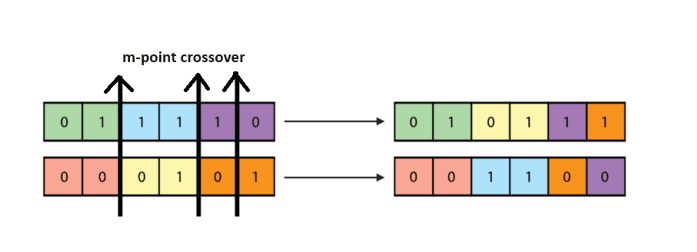
b. m-point crossover
The idea is same with 1-point crossover, we use m-point to cut each parent chromosome to (m + 1) part. The bits situated between the m points are swapped between the parent organisms.
Non-Linear crossover
This method is useful in case individuals in the population are permutations. A well-known representative of this problem is the traveling salesman problem (TSP) which aims to find the shortest path to visit a set of cities exactly once and return to the origin city. Partially mapped crossover (PMX), a method inspired by TSP, is specifically tailored for order-based permutations.
The partially mapped crossover (PMX):
Init 2 crossover points randomly
Their index is different with 0 and different with the length of chromosome – 1. These points divide the parents’ chromosomes into three segments: Left, middle, and right segmentation.
For example:

We fill the middle segmentation of the offspring corresponding to the middle of the parents' chromosomes with the rule above.
Fill the offspring remaining with the mapping relationship (The flow from left to right)
We commence with offspring 1, which requires filling two segments: The left segmentation and the right segmentation.
Now, let’s fill the left segment.
+ Starting with index 0, in the father's chromosome, gene 'A' represents this position. We verify if 'A' exists in offspring 1. If not, index 0 of offspring 1 is filled by ‘A’; otherwise, we must find a substitute for 'A'. Since 'A' is already present in offspring 1 at index 3. Index 3 in offspring 2 is gene ‘D’. Again, we check if 'D' exists in offspring 1. As it's already present, we cannot use 'D' to fill index 0 of offspring 1. 'D' corresponds to index 2 in offspring 2, where gene 'C' is located. And, 'C' has not yet present in offspring 1. Hence, we fill the first gene of offspring 1 with 'C'.
+ Moving to index 1, the father's chromosome holds gene 'B'. Since 'B' is not present in offspring 1, it occupies the second gene slot.
+ Repeat this process until reaching the last element of the first segment.
The same rule applies to completing the right segment.
In offspring 2, we follow the same process as in offspring 1, but we use the genetic material from the mother's chromosome instead.
Mutation
Mutation is the random alteration of bits on the chromosome string to generate diversity. For example, we have this chromosome: 10010100. The mutation occurred at indices 2 and 5, resulting in 10110000.
Mutation helps us escape local minima by enabling jumps to different regions of the search space. This allows for broader exploration and potentially leads to finding the global minimum.
Components in Genetic Algorithm
Initial population
The population contains many chromosomes. These initial chromosomes can be:
Generated randomly in the initial step
The results of other algorithms
Obtained by experts based on some specific conditions.
The number of chromosomes in the population is based on your resources.
Fitness function
The input of this function is the chromosomes and the output is the fitness value. This value shows us how close a candidate solution is to the optimal solution of the desired problem.
The fitness value is used for:
Select individuals who are a good fit for the next generation
Check the convergence of the algorithm
Termination condition
The termination is based on one of 3 criteria:
Fitness value: Once almost all candidate solutions in the population have the same fitness value, it means the algorithm convergence to a local minimum. You can stop the process.
Running time: The GA can stop after a predefined number of iterations. This decision depends on your available resources and desired execution time.
Diversity of the population: This diversity is measured by the variance of the candidate solutions. A low variance means these candidate solutions are generally similar and clustered together (convergence to a local minimum). A high variance tells us that the solutions have higher variability, and they are generally further from the mean.
Selection
Selection mechanisms are used to select candidate solutions to crossover for the next generation based on their fitness value. In general, we select the potentially useful solutions. Individuals whose high fitness value can be chosen. But it doesn’t mean we cross-over of two chromosomes have high fitness value we can get children with a high fitness value like their parents.
There are 4 methods for selection:
Roulette wheel Selection
This is the simplest way to select some solutions. Each individual has a part in Roulette wheel. The individual’s size in Roulette wheel directs proportion with the fitness value. Every time we spin the Roulette wheel we get one individual and consider it as a selected individual for regeneration.
For example, we have 5 chromosomes with their information as the table below:
The Roulette wheel of these chromosomes is like this:
We don't need to sort the percentages because we're aiming for random selection. In this method, we spin the roulette wheel n times to select n chromosomes. The probability of selecting a chromosome is directly proportional to its fitness value. This means chromosomes with higher fitness values have a greater chance of being selected. However, this can lead to a single chromosome being selected multiple times, potentially causing premature convergence to a local minimum.
Stochastic universal sampling Selection
The idea behind this method is similar to roulette wheel selection but with an improvement. The key difference lies in using pointers. Suppose we want to select 𝑚𝑚 chromosomes from a population of 𝑛 chromosomes. The first pointer is randomly generated. Then, we select the remaining 𝑚−1 chromosomes based on the distance between pointers [Equation] on a virtual roulette wheel.
Let's take a closer look at this example:
We need to select 3 chromosomes from a population of 5 chromosomes. The distance between pointers on the virtual roulette wheel is 1313 (120 degrees). Assume the first pointer randomly lands on chromosome_3. Therefore, the remaining 2 chromosomes selected are chromosome_2 and chromosome_0.
As you can see, we randomly generate only one pointer and then can choose k individuals. This method helps reduce duplication compared to roulette wheel selection.
Linear ranking Selection
Linear ranking selection employs a sorting approach to assign fitness value ranks. Individuals within the population are first ordered based on their fitness values decreasing, with the fittest receiving rank 1, the second fittest receiving rank 2, and so on until the lowest receives rank N (population size). The second step is selection, but how do we do that?
Tournament Selection
Randomly select k individuals ( k is called the tour size) and compare their fitness. The individual with the highest or lowest fitness or any standard based on your decision is chosen in each tour. This process is repeated n times with n as the number of individuals to be selected.
Crossover
Inspired by how genes mix in nature, genetic algorithms use crossover (also known as recombination) to generate new offspring from the genetic information of parents.
Linear crossover
This method is used for chromosome representation as a binary string.
1-point crossover
A random 'crossover point' is selected on both parents' chromosomes. At this point, the bits to the right are exchanged between the two parent chromosomes. Consequently, two offspring are produced, each inheriting genetic material from both parents.
b. m-point crossover
The idea is same with 1-point crossover, we use m-point to cut each parent chromosome to (m + 1) part. The bits situated between the m points are swapped between the parent organisms.
Non-Linear crossover
This method is useful in case individuals in the population are permutations. A well-known representative of this problem is the traveling salesman problem (TSP) which aims to find the shortest path to visit a set of cities exactly once and return to the origin city. Partially mapped crossover (PMX), a method inspired by TSP, is specifically tailored for order-based permutations.
The partially mapped crossover (PMX):
Init 2 crossover points randomly
Their index is different with 0 and different with the length of chromosome – 1. These points divide the parents’ chromosomes into three segments: Left, middle, and right segmentation.
For example:
We fill the middle segmentation of the offspring corresponding to the middle of the parents' chromosomes with the rule above.
Fill the offspring remaining with the mapping relationship (The flow from left to right)
We commence with offspring 1, which requires filling two segments: The left segmentation and the right segmentation.
Now, let’s fill the left segment.
+ Starting with index 0, in the father's chromosome, gene 'A' represents this position. We verify if 'A' exists in offspring 1. If not, index 0 of offspring 1 is filled by ‘A’; otherwise, we must find a substitute for 'A'. Since 'A' is already present in offspring 1 at index 3. Index 3 in offspring 2 is gene ‘D’. Again, we check if 'D' exists in offspring 1. As it's already present, we cannot use 'D' to fill index 0 of offspring 1. 'D' corresponds to index 2 in offspring 2, where gene 'C' is located. And, 'C' has not yet present in offspring 1. Hence, we fill the first gene of offspring 1 with 'C'.
+ Moving to index 1, the father's chromosome holds gene 'B'. Since 'B' is not present in offspring 1, it occupies the second gene slot.
+ Repeat this process until reaching the last element of the first segment.
The same rule applies to completing the right segment.
In offspring 2, we follow the same process as in offspring 1, but we use the genetic material from the mother's chromosome instead.
Mutation
Mutation is the random alteration of bits on the chromosome string to generate diversity. For example, we have this chromosome: 10010100. The mutation occurred at indices 2 and 5, resulting in 10110000.
Mutation helps us escape local minima by enabling jumps to different regions of the search space. This allows for broader exploration and potentially leads to finding the global minimum.
Case study
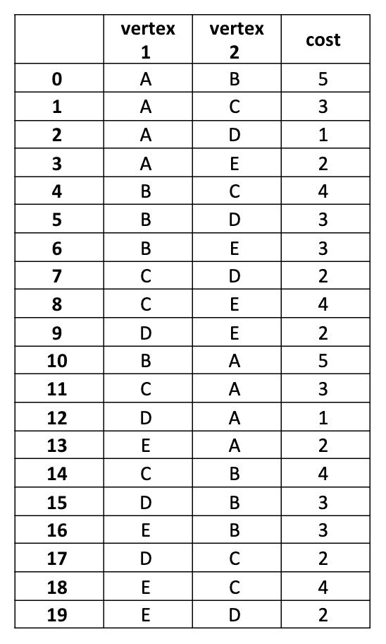
Traveling Salesman Problem (TSP)
Supposed we have a complete graph like this:

And we have to visit a set of all cities exactly once and then return to the origin city on the shortest tour.
Now, let’s build a TSP class!
import pandas as pd
import numpy as np  Create a data frame to store the weights of all paths in the graph class TSP:     def __init__(self, vertices, cost):         self.vertices = vertices         self.cost = cost         self.df = self.df_cost_lookup()      def df_cost_lookup(self):         v1 = []         v2 = []         for i in range(len(self.vertices)):             for j in range(i+1, len(self.vertices)):                 v1.append(self.vertices[i])                 v2.append(self.vertices[j])          data = {'vertex 1': v1 + v2, 'vertex 2': v2 + v1, 'cost': self.cost*2}          df = pd.DataFrame(data)
        return df
vertices = ['A', 'B', 'C', 'D', 'E']
cost = [5,3,1,2,4,3,3,2,4,2]
tsp_solver = TSP(vertices, cost)
tsp_solver.df_cost_lookup()
We get this result:
Define a function to calculate the cost of a path:
 def travel_cost_2_vertices(self, vertex_1, vertex_2):
        return self.df[(self.df['vertex 1'] == vertex_1) & (self.df['vertex 2'] == vertex_2)]['cost'].values[0]
def travel_cost(self, str_path):
        cost = 0
        for i in range(len(str_path)-1):
            vertex_1 = str_path[i]
            vertex_2 = str_path[i+1]
            cost += self.travel_cost_2_vertices(vertex_1, vertex_2)
        cost += self.travel_cost_2_vertices(str_path[-1], str_path[0])
        return cost
Implement a mutation function:
def swap(self, str_path, pos_1, pos_2):
        str_path = list(str_path)
        tmp = str_path[pos_1]
        str_path[pos_1] = str_path[pos_2]
        str_path[pos_2] = tmp
        return str_path

    def mutate(self, str_path):
        i, j = np.random.choice(list(range(0, len(str_path))), 2, replace=False)
        return self.swap(str_path, i, j)
Develop a crossover function (partially mapped crossover). The idea of this crossover method is presented in section 3.5.2
def find_duplicate_index(self, gene, str_path):
        for i in range(len(str_path)):
            if(str_path[i] == gene):
                return i

    def deductive(self, gene, child_1, child_2):
        while(gene in child_1):
            dup_idx = self.find_duplicate_index(gene, child_1)
            gene_2 = child_2[dup_idx]
            gene = gene_2
        return gene
def fill_chromosomes(self, str_path, child_1, child_2):
        for i in range(0, 2):
            gene_i = str_path[i]
            if(gene_i not in child_1):
                child_1[i] = gene_i
            else:
                gene_tmp = self.deductive(gene_i, child_1, child_2)
                child_1[i] = gene_tmp

        k = len(child_1) - 2 - 2 # 2 genes for the left and 2 genes for middle segmentation

        for j in range(k):
            gene_j = str_path[j+4]
            if(gene_j not in child_1):
                child_1[j+4] = gene_j
            else:
                gene_tmp = self.deductive(gene_j, child_1, child_2)
                child_1[j+4] = gene_tmp
        return child_1
def partially_mapped_crossover(self, str_path_1, str_path_2):
str_path_1 = list(str_path_1)
str_path_2 = list(str_path_2)
child_1 = ['0']*len(str_path_1)
child_2 = ['0']*len(str_path_2)
child_1[2:4] = str_path_2[2:4] # the middle segmentation get from mother’s chromosome
child_2[2:4] = str_path_1[2:4] # the middle segmentation get from father’s chromosome
child_1 = self.fill_chromosomes(str_path_1, child_1, child_2)
child_2 = self.fill_chromosomes(str_path_2, child_2, child_1)
return child_1, child_2
Init a population:
def init_population(self, population, start_vertex):
        travel_cost_lst = []
        path_lst = []
        for i in range(len(population)):
            str_path_i = population[i]

            for j in range(i+1, len(population)):

                str_path_1, str_path_2 = population[i], population[j]

                # Cross-over
                child_1, child_2 = self.partially_mapped_crossover(str_path_1, str_path_2)
                if(child_1[0] == start_vertex):
                # In the crossover process, the first gene may differ from the initial starting vertex
                # Therefore, each time a new chromosome is created, it is necessary to check whether the first gene of this chromosome coincides with the starting vertex.
                # If it does the new chromosome and the cost of movement are saved.

                    path_lst.append(child_1)
                    cost_1 = self.travel_cost(child_1)
                    travel_cost_lst.append(cost_1)
if(child_2[0] == start_vertex):
                    path_lst.append(child_2)
                    cost_2 = self.travel_cost(child_2)
                    travel_cost_lst.append(cost_2)
# Mutate
                child_1_mutate = self.mutate(child_1)
                child_2_mutate = self.mutate(child_2)

                if(child_1_mutate[0] == start_vertex):
                    path_lst.append(child_1_mutate)
                    cost_1_mutate = self.travel_cost(child_1_mutate)
                    travel_cost_lst.append(cost_1_mutate)
if(child_2_mutate[0] == start_vertex):
                    path_lst.append(child_2_mutate)
                    cost_2_mutate = self.travel_cost(child_2_mutate)
                    travel_cost_lst.append(cost_2_mutate)
population = []
        for x in np.asarray(path_lst)[np.argsort(travel_cost_lst)[0:3]]:
            x = ''.join(x)
            population.append(x)

        return population, path_lst, travel_cost_lst
Define a function to find the best path (The path with the lowest cost)
def find_best_path(self, path_lst, travel_cost_lst):
        min_cost = 100000
        min_path = None
        for i in range(len(travel_cost_lst)):
          if(travel_cost_lst[i] < min_cost):
            min_cost = travel_cost_lst[i]
            min_path = path_lst[i]
        return ''.join(min_path), min_cost
Suppose we start from vertex ‘D’. We need to create some elements for the initial population.
import itertools
import random

start_vertex = 'D' # Suppose we start from vertex 'D'
lst_tmp = list(itertools.permutations(['A', 'B', 'C', 'D', 'E']))
lst_tmp = lst_tmp[24*3:24*4] # each vertex has 24 paths start from it. This line of code aims to list all paths starting from 'D'

population_0 = [''.join(x) for x in random.sample(lst_tmp, 3)] # Initialize the initial population with 3 random elements population_1, path_lst_1, travel_cost_lst_1 = tsp_solver.init_population(population_0, start_vertex)In the first iteration, we get:
The top 3 elements with the best cost are: ['DAEBC', 'DEBCA', 'DAECB']
All paths generated in this iteration are: ['DABCE', 'DCABE', 'DABEC', 'DEABC', 'DCEAB', 'DEABC', 'DAECB', 'DAEBC', 'DCEAB', 'DEBCA', 'DEACB']
The corresponding cost: [16, 15, 15, 15, 16, 15, 14, 12, 16, 13, 14]
best_path_1, min_cost_1 = tsp_solver.find_best_path(path_lst_1, travel_cost_lst_1)The best path is ‘DAEBC’ and its cost is 12
The second iteration, we get
population_2, path_lst_2, travel_cost_lst_2 = tsp_solver.init_population(population_1, start_vertex)The top 3 elements with the best cost are: ['DAEBC', 'DAECB', 'DBECA']
All paths generated in this iteration are: ['DABCE', 'DCEBA', 'DAECB', 'DAEBC', 'DBECA', 'DBECA', 'DABCE', 'DABEC']
The corresponding path cost: [16, 15, 14, 12, 14, 14, 16, 15]
best_path_2, min_cost_2 = tsp_solver.find_best_path(path_lst_2, travel_cost_lst_2)The best path is ‘DAEBC’ and its cost is 12
(The result can be different each time we run the code)
Case study
Traveling Salesman Problem (TSP)
Supposed we have a complete graph like this:
And we have to visit a set of all cities exactly once and then return to the origin city on the shortest tour.
Now, let’s build a TSP class!
import pandas as pd
import numpy as np  Create a data frame to store the weights of all paths in the graph class TSP:     def __init__(self, vertices, cost):         self.vertices = vertices         self.cost = cost         self.df = self.df_cost_lookup()      def df_cost_lookup(self):         v1 = []         v2 = []         for i in range(len(self.vertices)):             for j in range(i+1, len(self.vertices)):                 v1.append(self.vertices[i])                 v2.append(self.vertices[j])          data = {'vertex 1': v1 + v2, 'vertex 2': v2 + v1, 'cost': self.cost*2}          df = pd.DataFrame(data)
        return df
vertices = ['A', 'B', 'C', 'D', 'E']
cost = [5,3,1,2,4,3,3,2,4,2]
tsp_solver = TSP(vertices, cost)
tsp_solver.df_cost_lookup()
We get this result:
Define a function to calculate the cost of a path:
 def travel_cost_2_vertices(self, vertex_1, vertex_2):
        return self.df[(self.df['vertex 1'] == vertex_1) & (self.df['vertex 2'] == vertex_2)]['cost'].values[0]
def travel_cost(self, str_path):
        cost = 0
        for i in range(len(str_path)-1):
            vertex_1 = str_path[i]
            vertex_2 = str_path[i+1]
            cost += self.travel_cost_2_vertices(vertex_1, vertex_2)
        cost += self.travel_cost_2_vertices(str_path[-1], str_path[0])
        return cost
Implement a mutation function:
def swap(self, str_path, pos_1, pos_2):
        str_path = list(str_path)
        tmp = str_path[pos_1]
        str_path[pos_1] = str_path[pos_2]
        str_path[pos_2] = tmp
        return str_path

    def mutate(self, str_path):
        i, j = np.random.choice(list(range(0, len(str_path))), 2, replace=False)
        return self.swap(str_path, i, j)
Develop a crossover function (partially mapped crossover). The idea of this crossover method is presented in section 3.5.2
def find_duplicate_index(self, gene, str_path):
        for i in range(len(str_path)):
            if(str_path[i] == gene):
                return i

    def deductive(self, gene, child_1, child_2):
        while(gene in child_1):
            dup_idx = self.find_duplicate_index(gene, child_1)
            gene_2 = child_2[dup_idx]
            gene = gene_2
        return gene
def fill_chromosomes(self, str_path, child_1, child_2):
        for i in range(0, 2):
            gene_i = str_path[i]
            if(gene_i not in child_1):
                child_1[i] = gene_i
            else:
                gene_tmp = self.deductive(gene_i, child_1, child_2)
                child_1[i] = gene_tmp

        k = len(child_1) - 2 - 2 # 2 genes for the left and 2 genes for middle segmentation

        for j in range(k):
            gene_j = str_path[j+4]
            if(gene_j not in child_1):
                child_1[j+4] = gene_j
            else:
                gene_tmp = self.deductive(gene_j, child_1, child_2)
                child_1[j+4] = gene_tmp
        return child_1
def partially_mapped_crossover(self, str_path_1, str_path_2):
str_path_1 = list(str_path_1)
str_path_2 = list(str_path_2)
child_1 = ['0']*len(str_path_1)
child_2 = ['0']*len(str_path_2)
child_1[2:4] = str_path_2[2:4] # the middle segmentation get from mother’s chromosome
child_2[2:4] = str_path_1[2:4] # the middle segmentation get from father’s chromosome
child_1 = self.fill_chromosomes(str_path_1, child_1, child_2)
child_2 = self.fill_chromosomes(str_path_2, child_2, child_1)
return child_1, child_2
Init a population:
def init_population(self, population, start_vertex):
        travel_cost_lst = []
        path_lst = []
        for i in range(len(population)):
            str_path_i = population[i]

            for j in range(i+1, len(population)):

                str_path_1, str_path_2 = population[i], population[j]

                # Cross-over
                child_1, child_2 = self.partially_mapped_crossover(str_path_1, str_path_2)
                if(child_1[0] == start_vertex):
                # In the crossover process, the first gene may differ from the initial starting vertex
                # Therefore, each time a new chromosome is created, it is necessary to check whether the first gene of this chromosome coincides with the starting vertex.
                # If it does the new chromosome and the cost of movement are saved.

                    path_lst.append(child_1)
                    cost_1 = self.travel_cost(child_1)
                    travel_cost_lst.append(cost_1)
if(child_2[0] == start_vertex):
                    path_lst.append(child_2)
                    cost_2 = self.travel_cost(child_2)
                    travel_cost_lst.append(cost_2)
# Mutate
                child_1_mutate = self.mutate(child_1)
                child_2_mutate = self.mutate(child_2)

                if(child_1_mutate[0] == start_vertex):
                    path_lst.append(child_1_mutate)
                    cost_1_mutate = self.travel_cost(child_1_mutate)
                    travel_cost_lst.append(cost_1_mutate)
if(child_2_mutate[0] == start_vertex):
                    path_lst.append(child_2_mutate)
                    cost_2_mutate = self.travel_cost(child_2_mutate)
                    travel_cost_lst.append(cost_2_mutate)
population = []
        for x in np.asarray(path_lst)[np.argsort(travel_cost_lst)[0:3]]:
            x = ''.join(x)
            population.append(x)

        return population, path_lst, travel_cost_lst
Define a function to find the best path (The path with the lowest cost)
def find_best_path(self, path_lst, travel_cost_lst):
        min_cost = 100000
        min_path = None
        for i in range(len(travel_cost_lst)):
          if(travel_cost_lst[i] < min_cost):
            min_cost = travel_cost_lst[i]
            min_path = path_lst[i]
        return ''.join(min_path), min_cost
Suppose we start from vertex ‘D’. We need to create some elements for the initial population.
import itertools
import random

start_vertex = 'D' # Suppose we start from vertex 'D'
lst_tmp = list(itertools.permutations(['A', 'B', 'C', 'D', 'E']))
lst_tmp = lst_tmp[24*3:24*4] # each vertex has 24 paths start from it. This line of code aims to list all paths starting from 'D'

population_0 = [''.join(x) for x in random.sample(lst_tmp, 3)] # Initialize the initial population with 3 random elements population_1, path_lst_1, travel_cost_lst_1 = tsp_solver.init_population(population_0, start_vertex)In the first iteration, we get:
The top 3 elements with the best cost are: ['DAEBC', 'DEBCA', 'DAECB']
All paths generated in this iteration are: ['DABCE', 'DCABE', 'DABEC', 'DEABC', 'DCEAB', 'DEABC', 'DAECB', 'DAEBC', 'DCEAB', 'DEBCA', 'DEACB']
The corresponding cost: [16, 15, 15, 15, 16, 15, 14, 12, 16, 13, 14]
best_path_1, min_cost_1 = tsp_solver.find_best_path(path_lst_1, travel_cost_lst_1)The best path is ‘DAEBC’ and its cost is 12
The second iteration, we get
population_2, path_lst_2, travel_cost_lst_2 = tsp_solver.init_population(population_1, start_vertex)The top 3 elements with the best cost are: ['DAEBC', 'DAECB', 'DBECA']
All paths generated in this iteration are: ['DABCE', 'DCEBA', 'DAECB', 'DAEBC', 'DBECA', 'DBECA', 'DABCE', 'DABEC']
The corresponding path cost: [16, 15, 14, 12, 14, 14, 16, 15]
best_path_2, min_cost_2 = tsp_solver.find_best_path(path_lst_2, travel_cost_lst_2)The best path is ‘DAEBC’ and its cost is 12
(The result can be different each time we run the code)
Dao Pham
Product Developer
#TechEnthusiast #AIProductDeveloper
Dao Pham
Product Developer
#TechEnthusiast #AIProductDeveloper
Dao Pham
Product Developer
#TechEnthusiast #AIProductDeveloper
Dao Pham
Product Developer
#TechEnthusiast #AIProductDeveloper