Annotab Studio 2.0.0 is now live
/
deep-learning-in-agriculture-advancing-leaf-analysis-with-classification-and-defect-detection-method
/
deep-learning-in-agriculture-advancing-leaf-analysis-with-classification-and-defect-detection-method
/
deep-learning-in-agriculture-advancing-leaf-analysis-with-classification-and-defect-detection-method
/
deep-learning-in-agriculture-advancing-leaf-analysis-with-classification-and-defect-detection-method
Deep Learning in Agriculture: Advancing Leaf Analysis with Classification and Defect Detection Method
Deep Learning in Agriculture: Advancing Leaf Analysis with Classification and Defect Detection Method
Deep Learning in Agriculture: Advancing Leaf Analysis with Classification and Defect Detection Method
Deep Learning in Agriculture: Advancing Leaf Analysis with Classification and Defect Detection Method
Published by

Dao Pham
on
Aug 8, 2023
under
Deep Learning
Published by
Dao Pham
on
Aug 8, 2023
under
Deep Learning
Published by
Dao Pham
on
Aug 8, 2023
under
Deep Learning
Published by
Dao Pham
on
Aug 8, 2023
under
Deep Learning
Tl;dr
Discover the transformative potential of deep learning in agriculture through image classification using VGG-19 and defect detection via color-based segmentation for enhanced crop analysis and management.
Tl;dr
Discover the transformative potential of deep learning in agriculture through image classification using VGG-19 and defect detection via color-based segmentation for enhanced crop analysis and management.
Tl;dr
Discover the transformative potential of deep learning in agriculture through image classification using VGG-19 and defect detection via color-based segmentation for enhanced crop analysis and management.
Tl;dr
Discover the transformative potential of deep learning in agriculture through image classification using VGG-19 and defect detection via color-based segmentation for enhanced crop analysis and management.

Introduction
In recent years, the field of agriculture has undergone a remarkable transformation with the introduction of deep learning techniques. These advanced methods, based on artificial intelligence (AI), have completely transformed agricultural practices and unlocked a world of opportunities for optimizing crop management. Leaf analysis plays a crucial role in plant identification, disease detection, and overall crop health assessment. While traditional methods relied on subjective manual inspection, with the integration of deep learning, we can now automate and enhance this process, significantly improving the accuracy and efficiency of the analysis.
In this article, we introduce a leaf analysis example with classification and defect detection.
Dataset
The dataset used in this study is Plant Leaves for Image Classification from Kaggle [1]. It consists of a comprehensive collection of leaf images from twelve selected plant species: Mango, Arjun, Alstonia Scholaris, Guava, Bael, Jamun, Jatropha, Pongamia Pinnata, Basil, Pomegranate, Lemon, and Chinar and classified. Images of both healthy and diseased leaves for each of these plant species (except Bael and Basil) were acquired and organized into separate modules. In the case of Bael and Basil, they especially have only one category: Bael diseased (P4b) and Basil healthy (P8).
The images were labeled based on the corresponding plant species, which were assigned names ranging from P0 to P11. The entire dataset was further divided into 22 subject categories, denoted as 0000 to 0022.
In this dataset, the classes labeled from 0000 to 0011 represent the healthy leaf class, while those labeled from 0012 to 0022 correspond to the diseased leaf class. The dataset comprises approximately 4,503 images, with 2,278 images belonging to the healthy leaf category and 2,225 images representing the diseased leaf category.
Before we start, it’s important to note that this dataset is shared under the Community Data License Agreement - Sharing - Version 1.0. The license provides guidelines and permissions for sharing and using the dataset in a professional setting.
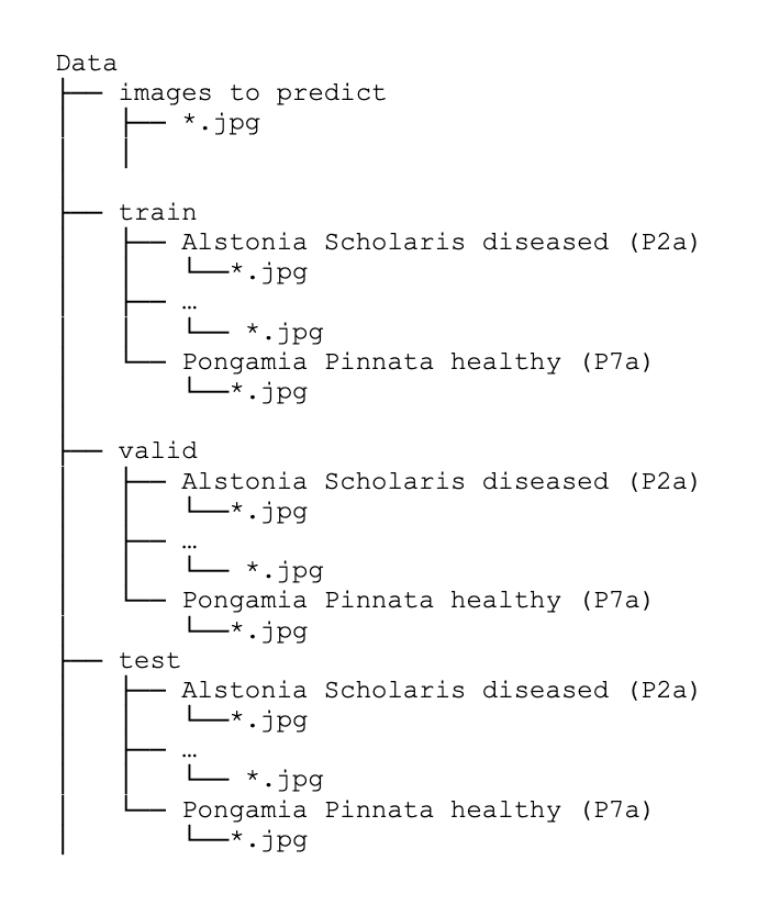
Once we download the dataset and unzip it, the following directory structure appears:
Then, let's get started.
Dataset
The dataset used in this study is Plant Leaves for Image Classification from Kaggle [1]. It consists of a comprehensive collection of leaf images from twelve selected plant species: Mango, Arjun, Alstonia Scholaris, Guava, Bael, Jamun, Jatropha, Pongamia Pinnata, Basil, Pomegranate, Lemon, and Chinar and classified. Images of both healthy and diseased leaves for each of these plant species (except Bael and Basil) were acquired and organized into separate modules. In the case of Bael and Basil, they especially have only one category: Bael diseased (P4b) and Basil healthy (P8).
The images were labeled based on the corresponding plant species, which were assigned names ranging from P0 to P11. The entire dataset was further divided into 22 subject categories, denoted as 0000 to 0022.
In this dataset, the classes labeled from 0000 to 0011 represent the healthy leaf class, while those labeled from 0012 to 0022 correspond to the diseased leaf class. The dataset comprises approximately 4,503 images, with 2,278 images belonging to the healthy leaf category and 2,225 images representing the diseased leaf category.
Before we start, it’s important to note that this dataset is shared under the Community Data License Agreement - Sharing - Version 1.0. The license provides guidelines and permissions for sharing and using the dataset in a professional setting.
Once we download the dataset and unzip it, the following directory structure appears:
Then, let's get started.
Method
Leaf Classification
Exploratory Data Analysis (EDA)
First, we begin by importing essential libraries and modules required for deep learning in image analysis tasks.
from tensorflow import keras
import matplotlib.pyplot as plt
from keras import backend as k
import numpy as np
import os
import cv2
Subsequently, moving to proceed with conducting exploratory data analysis.
We encode the names of the plant species using label encoding technique. This process involves converting the names of the twelve classes into corresponding numerical representations.
folder_train = ‘path_to_ train’
class_folders_train = sorted(os.listdir(folder_train))Output:
class_folders_train = ['Alstonia Scholaris diseased (P2a)', 'Alstonia Scholaris healthy (P2b)', 'Arjun diseased (P1a)', 'Arjun healthy (P1b)', 'Bael diseased (P4b)', 'Basil healthy (P8)', 'Chinar diseased (P11b)', 'Chinar healthy (P11a)', 'Gauva diseased (P3b)', 'Gauva healthy (P3a)', 'Jamun diseased (P5b)', 'Jamun healthy (P5a)', 'Jatropha diseased (P6b)', 'Jatropha healthy (P6a)', 'Lemon diseased (P10b)', 'Lemon healthy (P10a)', 'Mango diseased (P0b)', 'Mango healthy (P0a)', 'Pomegranate diseased (P9b)', 'Pomegranate healthy (P9a)', 'Pongamia Pinnata diseased (P7b)', 'Pongamia Pinnata healthy (P7a)']label_mapping = {}
for i, class_folder in enumerate(class_folders_train):
label_mapping[i] = class_folder
display(label_mapping)Let's explore the result of this encoding process by examining the transformed data.
{0: 'Alstonia Scholaris diseased (P2a)',
1: 'Alstonia Scholaris healthy (P2b)',
2: 'Arjun diseased (P1a)',
3: 'Arjun healthy (P1b)',
4: 'Bael diseased (P4b)',
5: 'Basil healthy (P8)',
6: 'Chinar diseased (P11b)',
7: 'Chinar healthy (P11a)',
8: 'Gauva diseased (P3b)',
9: 'Gauva healthy (P3a)',
10: 'Jamun diseased (P5b)',
11: 'Jamun healthy (P5a)',
12: 'Jatropha diseased (P6b)',
13: 'Jatropha healthy (P6a)',
14: 'Lemon diseased (P10b)',
15: 'Lemon healthy (P10a)',
16: 'Mango diseased (P0b)',
17: 'Mango healthy (P0a)',
18: 'Pomegranate diseased (P9b)',
19: 'Pomegranate healthy (P9a)',
20: 'Pongamia Pinnata diseased (P7b)',
21: 'Pongamia Pinnata healthy (P7a)'}
In the next step, we conduct data exploration by randomly choosing one image from each species and plotting it to provide a summarized visual representation. This step allows us to gain an initial understanding of the characteristics exhibited by each plant species.
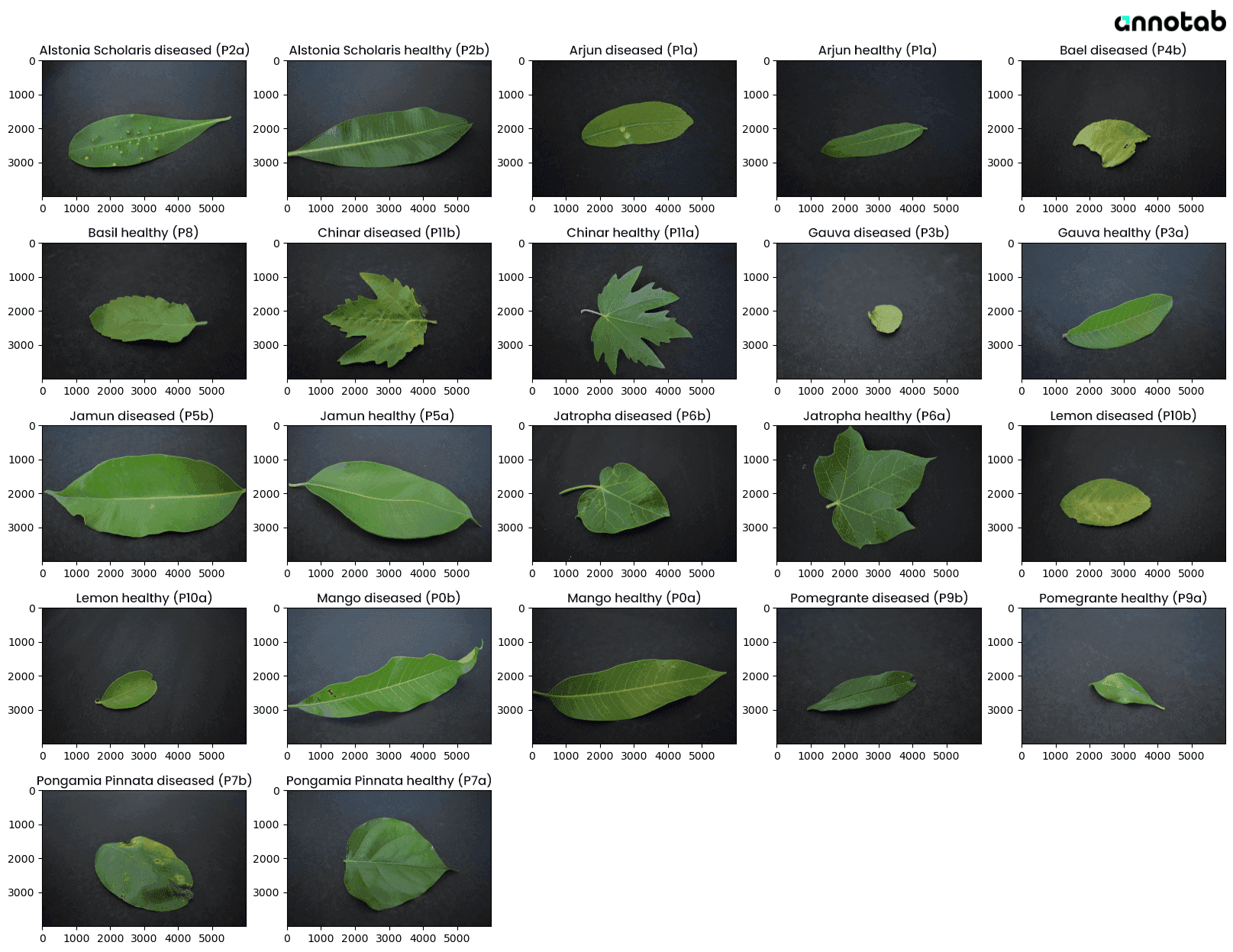
Figure 1: Random image samples from twelve plant species
To plot this, you can use the following lines of code:
visualized_data = []
for i in range(len(class_folders_train)):
    image_name = random.choice(os.listdir(folder_train + class_folders_train[i]))
    image = cv2.imread(os.path.join(folder_train, class_folders_train[i], image_name))
    visualized_data.append(cv2.cvtColor(image, cv2.COLOR_BGR2RGB))
fig = plt.figure(figsize=(20, 15))
columns = 5
rows = 5
for i in range(1, columns*rows):
if (i < len(visualized_data)+1):
image = visualized_data[i-1]
fig.add_subplot(rows, columns, i)
plt.title(class_folders_train[i-1])
plt.imshow(image)
plt.show()In addition, we created a bar chart to represent the number of plants in two distinct states: "diseases" and "healthy”. To do this, we need to count the number in two states of each species:
class_folders_train_temp = [x for x in class_folders_train if x not in ['Bael diseased (P4b)', 'Basil healthy (P8)']]
diseased  = []
healthy  = []
for i in range(len(class_folders_train_temp)):
    class_i = class_folders_train_temp[i]
    num_class_i = len(os.listdir(folder_train + class_i))
    if (i % 2 == 0):
        diseased.append(num_class_i)
    else:
healthy.append(num_class_i)plant_species.append('Basil')
healthy.append(len(os.listdir(folder_train + 'Basil healthy (P8)')))
diseased.append(0)
plant_species.append('Bael')
healthy.append(0)
diseased.append(len(os.listdir(folder_train + 'Bael diseased (P4b)')))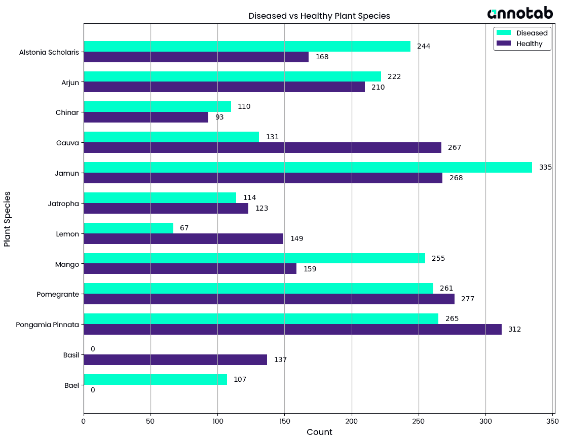
Figure 2: Health Condition Distribution: Plants in Diseased and Healthy States
This chart aims to provide a comparison by illustrating the distribution of twelve plant species across two states of health conditions. The bars representing the "diseases" state indicate the number of plants within each species that are affected by diseases or experiencing some form of health issues. The bars representing the "healthy" state indicate the number of plants within each species that are in good health and free from any noticeable diseases or health problems. At first glance, we can observe that the distribution of the two states within the same species is imbalanced. Furthermore, the number of samples across different plant species is also uneven. Additionally, Basil and Bael are two specific cases worth noting: Basil does not have any samples in the diseased state, while Bael does not have any samples in the healthy state.
Network Details
The neural network created in this case uses the Tensorflow architecture. The VGG-19 [2] neural network is used.
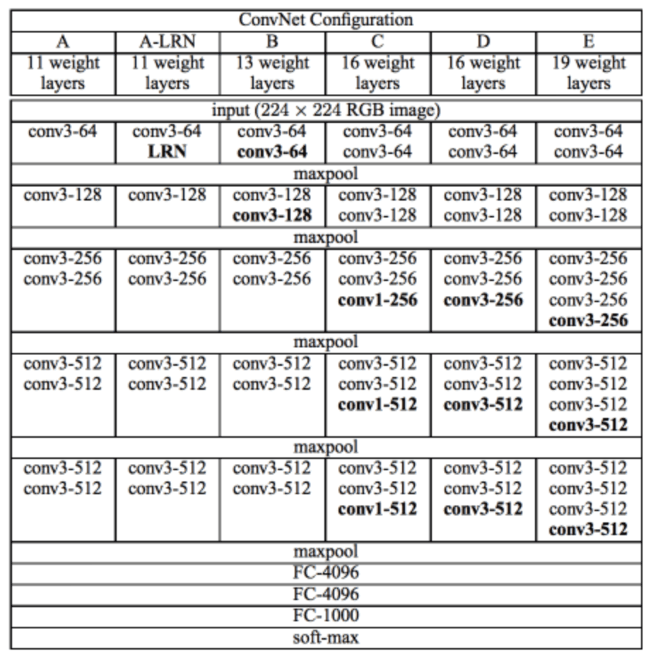
Figure 3: VGG-19 architecture
After completing the model training process, we will utilize the trained model to generate predictions on both the validation set and the test set. This step allows us to thoroughly assess the performance and accuracy of the model. The accuracy of validation set and testing set provide valuable insights into the model's ability to generalize to unseen data and its overall effectiveness in solving the given problem.
# Load the model that is saved after the training process
model.load_weights("path_to_model_checkpoint")

# Evaluate the model on the valid set
valid_loss, valid_accuracy = model.evaluate(valid_generator, steps=len(valid_generator))
print("Valid Loss:", valid_loss)
print("Valid Accuracy:", valid_accuracy)

# Evaluate the model on the test set
test_loss, test_accuracy = model.evaluate(test_generator, steps=len(test_generator))
print("Test Loss:", test_loss)
print("Test Accuracy:", test_accuracy)Output:
4/4 [==============================] - 17s 4s/step - loss: 0.6710 - accuracy: 0.7636
Valid Loss: 0.671012818813324
Valid Accuracy: 0.7636363506317139
4/4 [==============================] - 17s 4s/step - loss: 0.6784 - accuracy: 0.7455
Test Loss: 0.6784456968307495
Test Accuracy: 0.7454545497894287Now, let's examine the results. The results indicate that the model achieved an accuracy of 76.4% on the validation set and 74.5% on the testing set. Additionally, the F1-score obtained on the test set is 0.7376. Considering the complexity of multiclass classification involving 22 classes and potential data imbalance, this F1-score is considered to be reasonably good. It indicates that the model effectively achieves a balance between accurately identifying positive samples (precision) and appropriately capturing positive samples (recall).

Figure 4: Confusion Matrix for 22 Classes on Testing Set
Leaf Defect Detection
We are now ready to evaluate the model using images in 'image to predict' folder. This folder consists of 8 unlabeled images.
The main idea of defect detection in this scenario is using the color-based approach by identifying areas on the leaf that lie outside the green color range since the majority of the healthy leaf in this dataset exhibit green coloration. The process involves the following steps:
(1) First, classify leaf images to determine their respective classes and identify whether they are diseased or healthy.

Figure 5: Leaf Image Analysis: Predicted Labels
(2) In the second step, if the leaf image is diseased, I’ll detect the region of the defect. To achieve this, I use the Segment Anything Model (SAM) from Meta [3] to “cut out” the leaf and remove the image’s background. This step is essential because we rely on the leaf’s color to detect defective regions, and thus, removing the background is necessary. Next, I segment the defective regions based on the main idea mentioned above. This will yield the final result: The identification of defective regions on the leaf.

Figure 6: Leaf Image Analysis: Defective Region Segmentation
Method
Leaf Classification
Exploratory Data Analysis (EDA)
First, we begin by importing essential libraries and modules required for deep learning in image analysis tasks.
from tensorflow import keras
import matplotlib.pyplot as plt
from keras import backend as k
import numpy as np
import os
import cv2
Subsequently, moving to proceed with conducting exploratory data analysis.
We encode the names of the plant species using label encoding technique. This process involves converting the names of the twelve classes into corresponding numerical representations.
folder_train = ‘path_to_ train’
class_folders_train = sorted(os.listdir(folder_train))Output:
class_folders_train = ['Alstonia Scholaris diseased (P2a)', 'Alstonia Scholaris healthy (P2b)', 'Arjun diseased (P1a)', 'Arjun healthy (P1b)', 'Bael diseased (P4b)', 'Basil healthy (P8)', 'Chinar diseased (P11b)', 'Chinar healthy (P11a)', 'Gauva diseased (P3b)', 'Gauva healthy (P3a)', 'Jamun diseased (P5b)', 'Jamun healthy (P5a)', 'Jatropha diseased (P6b)', 'Jatropha healthy (P6a)', 'Lemon diseased (P10b)', 'Lemon healthy (P10a)', 'Mango diseased (P0b)', 'Mango healthy (P0a)', 'Pomegranate diseased (P9b)', 'Pomegranate healthy (P9a)', 'Pongamia Pinnata diseased (P7b)', 'Pongamia Pinnata healthy (P7a)']label_mapping = {}
for i, class_folder in enumerate(class_folders_train):
label_mapping[i] = class_folder
display(label_mapping)Let's explore the result of this encoding process by examining the transformed data.
{0: 'Alstonia Scholaris diseased (P2a)',
1: 'Alstonia Scholaris healthy (P2b)',
2: 'Arjun diseased (P1a)',
3: 'Arjun healthy (P1b)',
4: 'Bael diseased (P4b)',
5: 'Basil healthy (P8)',
6: 'Chinar diseased (P11b)',
7: 'Chinar healthy (P11a)',
8: 'Gauva diseased (P3b)',
9: 'Gauva healthy (P3a)',
10: 'Jamun diseased (P5b)',
11: 'Jamun healthy (P5a)',
12: 'Jatropha diseased (P6b)',
13: 'Jatropha healthy (P6a)',
14: 'Lemon diseased (P10b)',
15: 'Lemon healthy (P10a)',
16: 'Mango diseased (P0b)',
17: 'Mango healthy (P0a)',
18: 'Pomegranate diseased (P9b)',
19: 'Pomegranate healthy (P9a)',
20: 'Pongamia Pinnata diseased (P7b)',
21: 'Pongamia Pinnata healthy (P7a)'}
In the next step, we conduct data exploration by randomly choosing one image from each species and plotting it to provide a summarized visual representation. This step allows us to gain an initial understanding of the characteristics exhibited by each plant species.
Figure 1: Random image samples from twelve plant species
To plot this, you can use the following lines of code:
visualized_data = []
for i in range(len(class_folders_train)):
    image_name = random.choice(os.listdir(folder_train + class_folders_train[i]))
    image = cv2.imread(os.path.join(folder_train, class_folders_train[i], image_name))
    visualized_data.append(cv2.cvtColor(image, cv2.COLOR_BGR2RGB))
fig = plt.figure(figsize=(20, 15))
columns = 5
rows = 5
for i in range(1, columns*rows):
if (i < len(visualized_data)+1):
image = visualized_data[i-1]
fig.add_subplot(rows, columns, i)
plt.title(class_folders_train[i-1])
plt.imshow(image)
plt.show()In addition, we created a bar chart to represent the number of plants in two distinct states: "diseases" and "healthy”. To do this, we need to count the number in two states of each species:
class_folders_train_temp = [x for x in class_folders_train if x not in ['Bael diseased (P4b)', 'Basil healthy (P8)']]
diseased  = []
healthy  = []
for i in range(len(class_folders_train_temp)):
    class_i = class_folders_train_temp[i]
    num_class_i = len(os.listdir(folder_train + class_i))
    if (i % 2 == 0):
        diseased.append(num_class_i)
    else:
healthy.append(num_class_i)plant_species.append('Basil')
healthy.append(len(os.listdir(folder_train + 'Basil healthy (P8)')))
diseased.append(0)
plant_species.append('Bael')
healthy.append(0)
diseased.append(len(os.listdir(folder_train + 'Bael diseased (P4b)')))Figure 2: Health Condition Distribution: Plants in Diseased and Healthy States
This chart aims to provide a comparison by illustrating the distribution of twelve plant species across two states of health conditions. The bars representing the "diseases" state indicate the number of plants within each species that are affected by diseases or experiencing some form of health issues. The bars representing the "healthy" state indicate the number of plants within each species that are in good health and free from any noticeable diseases or health problems. At first glance, we can observe that the distribution of the two states within the same species is imbalanced. Furthermore, the number of samples across different plant species is also uneven. Additionally, Basil and Bael are two specific cases worth noting: Basil does not have any samples in the diseased state, while Bael does not have any samples in the healthy state.
Network Details
The neural network created in this case uses the Tensorflow architecture. The VGG-19 [2] neural network is used.
Figure 3: VGG-19 architecture
After completing the model training process, we will utilize the trained model to generate predictions on both the validation set and the test set. This step allows us to thoroughly assess the performance and accuracy of the model. The accuracy of validation set and testing set provide valuable insights into the model's ability to generalize to unseen data and its overall effectiveness in solving the given problem.
# Load the model that is saved after the training process
model.load_weights("path_to_model_checkpoint")

# Evaluate the model on the valid set
valid_loss, valid_accuracy = model.evaluate(valid_generator, steps=len(valid_generator))
print("Valid Loss:", valid_loss)
print("Valid Accuracy:", valid_accuracy)

# Evaluate the model on the test set
test_loss, test_accuracy = model.evaluate(test_generator, steps=len(test_generator))
print("Test Loss:", test_loss)
print("Test Accuracy:", test_accuracy)Output:
4/4 [==============================] - 17s 4s/step - loss: 0.6710 - accuracy: 0.7636
Valid Loss: 0.671012818813324
Valid Accuracy: 0.7636363506317139
4/4 [==============================] - 17s 4s/step - loss: 0.6784 - accuracy: 0.7455
Test Loss: 0.6784456968307495
Test Accuracy: 0.7454545497894287Now, let's examine the results. The results indicate that the model achieved an accuracy of 76.4% on the validation set and 74.5% on the testing set. Additionally, the F1-score obtained on the test set is 0.7376. Considering the complexity of multiclass classification involving 22 classes and potential data imbalance, this F1-score is considered to be reasonably good. It indicates that the model effectively achieves a balance between accurately identifying positive samples (precision) and appropriately capturing positive samples (recall).
Figure 4: Confusion Matrix for 22 Classes on Testing Set
Leaf Defect Detection
We are now ready to evaluate the model using images in 'image to predict' folder. This folder consists of 8 unlabeled images.
The main idea of defect detection in this scenario is using the color-based approach by identifying areas on the leaf that lie outside the green color range since the majority of the healthy leaf in this dataset exhibit green coloration. The process involves the following steps:
(1) First, classify leaf images to determine their respective classes and identify whether they are diseased or healthy.
Figure 5: Leaf Image Analysis: Predicted Labels
(2) In the second step, if the leaf image is diseased, I’ll detect the region of the defect. To achieve this, I use the Segment Anything Model (SAM) from Meta [3] to “cut out” the leaf and remove the image’s background. This step is essential because we rely on the leaf’s color to detect defective regions, and thus, removing the background is necessary. Next, I segment the defective regions based on the main idea mentioned above. This will yield the final result: The identification of defective regions on the leaf.
Figure 6: Leaf Image Analysis: Defective Region Segmentation
Conclusion
Generally, the result is regarded acceptable as it successfully covers most of the defective areas. However, there is a drawback to this approach as it also considers the petiole, vein, and midrib as defective regions solely due to their color being outside the green range, although they are not in this case. Please note that utilizing colors within the green range to detect defects is a straightforward method.
In case the healthy leaves in your dataset do not have a green color, you can determine the color range for each healthy species. With a test leaf image, the first step is to classify it, and if it is diseased, follow the steps mentioned above, aligning with the corresponding plant species. Alternatively, you can explore another approach that aligns better with your specific objectives.
(You can find the complete code and the trained model checkpoint here).
References
[1] csafrit2. (2022). Plant Leaves for Image Classification. Kaggle. Community Data License Agreement - Sharing - Version 1.0. https://www.kaggle.com/datasets/csafrit2/plant-leaves-for-image-classification
[2] K. Simonyan and A. Zisserman. Very Deep Convolutional Networks for Large-Scale Image Recognition. arXiv:1409.1556 [cs.CV], 2014.
[3] Alexander Kirillov, Eric Mintun, Nikhila Ravi, Hanzi Mao, Chloe Rolland, Laura Gustafson, Tete Xiao, Spencer Whitehead, Alexander C. Berg, Wan-Yen Lo, Piotr Dollár, Ross Girshick. "Segment Anything." arXiv:2304.02643 [cs.CV], 2023
Read more
Dao Pham
Product Developer
#TechEnthusiast #AIProductDeveloper
Dao Pham
Product Developer
#TechEnthusiast #AIProductDeveloper
Dao Pham
Product Developer
#TechEnthusiast #AIProductDeveloper
Dao Pham
Product Developer
#TechEnthusiast #AIProductDeveloper